Expert Commentary

Recently, a company needed to forecast mid- and long-term effects of changes in local commodity prices critical to its country’s economy. We were asked to develop a software solution that would consider the effects on the total economy as well as on the individual sectors, such as imports and exports. The company wanted to review and compare outcomes of different commodity-price-change scenarios, in order to make better-informed strategic decisions.
The scope and complexity of the project required collaboration among data scientists, econometricians, and economists with expert knowledge of the local market. Gathering these different types of expertise was critical to developing robust models and software applications.
Challenges of economic time series forecasting
After evaluating various analytical approaches, the team decided to use a forecasting technique called a sign-restricted Bayesian vector autoregression (BVAR) model. That decision addressed several aspects of this project:
- Market dynamics stem from the interaction of many economic variables, none of which should be modeled on its own. In such situations, you must simulate how time-dependent variables affect one another. VARs do this by simultaneously modeling a number of interdependent equations, so that each variable serves as both a time-dependent output of a particular equation, as well as input for other equations.
- Data for training and validating models is limited. Many economic variables in this particular country have been captured only annually, and do not extend far into the past. Machine learning experts know that training complex models on insufficient amounts of data results in overfitting, which infects the model with errors and lowers the quality of the forecast. Bayesian models contain hyperparameters that regulate the effective size of the space across which the model parameters are optimized. This allows you to tune the complexity of these models, making them more robust, thus reducing the risk of overfitting.
- The available data also has little historical variance. This makes it difficult for the algorithm to learn relationships between the variables. Sign-restricted Bayesian methods provide a natural framework for incorporating expert knowledge about interdependencies between economic variables into such a system of equations.
Preparing the data and building the model
A typical machine-learning process involves several stages, each essential to obtaining trustworthy results. Typical stages include selecting the right modeling approach, data preprocessing and feature engineering, correctly setting up the training process, and careful model tuning and validation.
Moreover, in the context of economic forecasting in the presence of interdependent variables, many of these stages require market expertise. This is especially relevant with sign-restricted BVARs, where the market expert provides insights around the relationship expectations among the economic indicators. For example, an economist can determine the nature of a relationship between two economic variables (independent, cause-effect or mutually dependent) or provide input on what level of time-lagged effects are realistic in the local market. These insights would be factored later into the hyperparameter tuning.
Several other decisions come up during the modeling process:
- You may need to assess and potentially correct issues arising in time series forecasting, such as nonstationarity, variables co-integration and training data. These have effects on the model quality, especially its long-term stability.
- Monetary variables usually are provided in nominal values, and should be converted to real values in order to account for the effects of inflation.
- While optional, consider converting monetary economic variables from their original currencies to one chosen currency, such as US dollars. This allows you to link local market dynamics to the global economy.
- Specific to macroeconomic modeling, it’s important to ensure consistency between the total economy and individual sectors. We took a top-down approach, by modeling the total economy separately from the sectors, then connecting the two sides through a scaling factor.
The role of impulse response functions
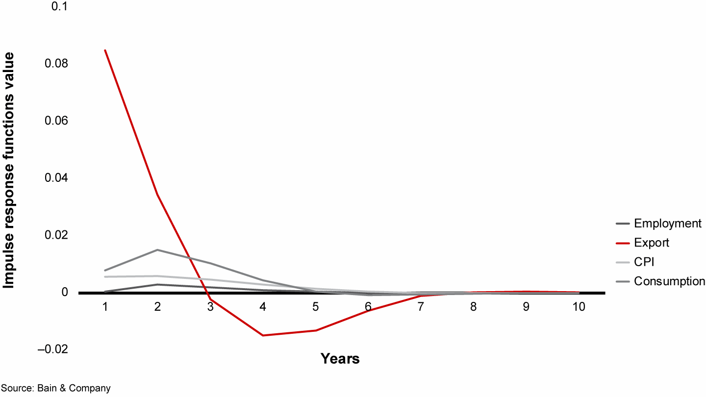
Once we trained the model and computed forecasts, the next step was to modify this forecast by taking into account various price-change scenarios. The key outputs of the training process that enable this are impulse response functions (IRFs).
The IRFs show how a one-time unit shock in one of the variables affects the others. By modeling several shocks in the different commodity prices, we could evaluate the mid- and long-term predictions of economic variables in each of the sectors and in the total economy (see Figure 1).


The IRFs also serve as a good indicator of model quality: In a correctly built model, the IRFs should smoothly decay to zero over time. If this isn’t reflected in the IRFs, that indicates the model does not have long-term stability.
The tool we built allows the user to model scenarios where different commodities undergo different tunable price changes. It then combines the IRFs with the corresponding commodity prices and shows the user the dynamics of the economy in this particular scenario. Being able to simulate and compare different scenarios allows the company to make smart business decisions amid changing market conditions.
* * *
By choosing appropriate data preprocessing steps and the right modeling approach—sign-restricted BVARS in this case—you can overcome the limitations imposed by small amounts of historical data. Delivering the model through a bespoke software solution allows you to design a user-friendly interface. This gives users flexibility to perform economic scenario modeling without being experts in the specific domain.